Hiding Cell Values In Excel
I have an Excel spreadsheet that I use to keep track of all my business expenses. In order to make it less cluttered, and easier on the eye, I wanted to get rid of all the repeated, irrelevant values in the columns that may not have an entry for each day. Here I am using a subset of the data, but it illustrates what I am trying to achieve:
| Date | Miles | Cumulative |
|---|---|---|
| 02/03/2020 | 3790 | |
| 03/03/2020 | 150 | 3940 |
| 04/03/2020 | 3940 | |
| 05/03/2020 | 3940 | |
| 06/03/2020 | 150 | 4090 |
| 07/03/2020 | 4090 | |
| 08/03/2020 | 4090 |
Hiding zero values in a range or even a whole worksheet is easy. However, I wanted to hide the value of a cell if its neighbouring cell is zero or blank. Here’s how I did it:
Select the values in the column you wish values to be hidden (“Cumulative” in this case).
On the Home toolbar click the “Conditional Formatting” button, select “Highlight Cells Rules” then “More Rules…”
Ensure the Style is “Classic” and then select “Use a formula to determine which cells to format” in the drop-down. Enter “=$b2=0” in the text box. Obviously, my data is in Column B and starts in Row 2, so you will need to to adjust this as necessary.
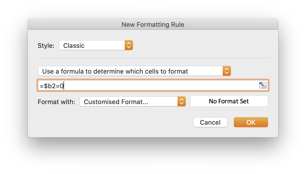
In the “Format with” drop-down select “Customised Format…”
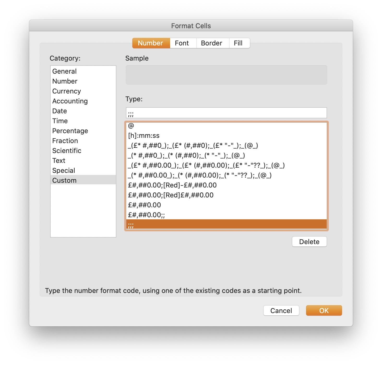
Select “Custom” under “Category” and then select (or enter) “;;;” for the “Type”
- Select “OK” twice
The “Cumulative” column now only shows data where there is an entry for that row in the “Miles” column:
| Date | Miles | Cumulative |
|---|---|---|
| 02/03/2020 | ||
| 03/03/2020 | 150 | 3940 |
| 04/03/2020 | ||
| 05/03/2020 | ||
| 06/03/2020 | 150 | 4090 |
| 07/03/2020 | ||
| 08/03/2020 |